THE CHAOS THEORY:
CHAOTIC SYSTEMS
(April 2025)
ABSTRACT
Chaotic systems are by definition systems with unpredictable behavior, memoryless systems. The already known chaotic systems are deterministic, labile systems, their behavior depends on the initial value, and after a finite time their behavior becomes chaotic and unpredictable. The chaotic behavior is an internal (immanent) property of chaotic systems, and chaotic behavior can only be described by probabilistic, stochastic means. New chaotic systems, e.g. related to waiting times, random walk problems, random numbers, random graphs, are described by the concepts of memorylessness, unpredictable behavior, and independent incremental, additive processes. In memoryless systems, the future of the eternally young process is independent of the present and past of the process, which have exponential or geometric distributions. Stochastic processes with independent increments are called memoryless, unpredictable processes. Chaotic systems are often related to the length of lifetimes, waiting times, and generally random periods of time until some event occurs.
In the normal distribution, the expected value and the standard deviation are independent quantities, while at the uniform distribution, the zero expected value and the standard deviation, the range, are independent. In the Kalman filter, a white Gaussian process with zero expected value, or a white noise process with zero expected value, is assumed. In vector linear analysis, the conditional expected value and the noise process associated with chaotic behavior are perpendicular to each other, which allows for a simple discussion of unpredictable, chaotic systems: the conditional expected value vector is perpendicular to the estimation error. In an exponential or geometric distribution, the past and present of the processes are perpendicular to their future.

London sculpture about random wandering (https://en.wikipedia.org/wiki/Random_walk)
INTRODUCTION
The well-known chaos theory (https://hu.wikipedia.org/wiki/K%C3%A1oszelm%C3%A9let) deals with nonlinear deterministic time-dependent and unstable systems whose behaviour can be only partially predicted, despite the deterministic regularities. The considered labile systems are sensitive to initial conditions, also known as butterfly effect. Unstable deterministic systems can be partially described by statistical, stochastic methods, not necessarily because they are complicated, but because chaotic behaviour is an intrinsic property of the systems, and after a finite time their behaviour becomes independent of initial conditions.
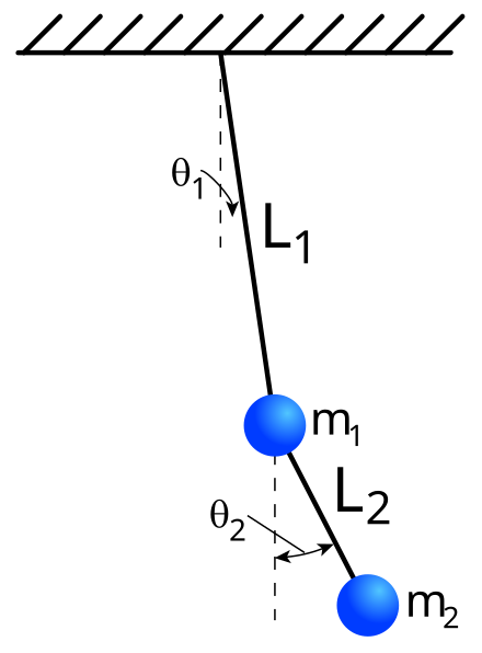
For real deterministic systems, asymptotic behaviour is clearly defined at t = infinity, i.e. only partially deterministic unstable systems can behave chaotically. Deterministic systems that can be described by few state labels may also exhibit unpredictable behaviour. For example, the motion of a double pendulum becomes independent of its initial state after a certain time, it does not return to its initial state, it is structurally unstable:

A double pendulum is a simple physical system consisting of two pendulums attached to each other, whose chaotic motion is initially governed by deterministic differential equations, but after a while its motion becomes random and chaotic. There are several variants, the length and mass of the two pendulums can be the same or different(https://scienceworld.wolfram.com/physics/DoublePendulum.html). The description of the motion can be either 3-dimensional or 2-dimensional.
.
The considered systems with chaotic behaviour are only partially deterministic systems, in contrast to the meaning of the word chaos means complete randomness (uncorrelated, possibly independent processes). After a finite time, instability, local disorder, characterises the chaotic systems. Behaviour is locally unstable if, starting from two starting positions close to each other, the differences between the states of the system increase in finite time in an unmodelled, unpredictable way. In 1961, the American meteorologist Edward Lorenz used a computer (Royal-McBee LGP-30), now considered very slow, to test his three-degree-of-freedom nonlinear convection model. On one occasion he wanted to recalculate a data series and to save time, he fed the output of an earlier simulation back into the computer. The new result quickly diverged from the last one. He suspected a computer error, but as he discovered, the computer was not at fault. The computer was plotting the data to 6 decimal places, but Lorenz was only writing it back to the machine to 3 decimal places. This small inaccuracy caused the very large discrepancy. In a 1963 paper, Edward Lorenz recognised the high sensitivity of nonlinear deterministic systems to small deviations in initial conditions. The phenomenon is often cited as the butterfly effect, based on the title of one of his lectures, Predictability: Does the flap of a butterfly's wings in Brazil set off a tornado in Texas? Small variations in the initial conditions cause unmodelable large changes in the state of an labile system - a system in an labile equilibrium state - and therefore long-term prediction of its behaviour is impossible, which is a fundamental property of labile systems.
The word chaos was introduced by Tien Yien Li and James A. Yorke in their 1975 article Period three implies chaos... "According to the Japan Foundation for Science and Technology, Yorke received the award for his work in the study of chaotic systems, while Mandelbrot received the award for his work on fractals. Although the Japan Prize is less well known in the public consciousness than the Nobel Prize and the Fields Medal, which are announced and awarded with increased media attention, the prize, which carries a cash award of $412 000, is hardly less recognised in scientific circles than the latter." There is an area of physics called quantum chaos theory, another chapter of chaos theory that deals with non-deterministic systems following the laws of quantum mechanics and another chapter where the behaviour of systems is unpredictable and systems can only be described by statistical, probabilistic methods.
There is a field of physics called quantum chaos theory, another chapter of chaos theory, which deals with non-deterministic systems following the laws of quantum mechanics Another new chapter of chaos theory, when the behavior of systems is unpredictable, and the systems can be described exclusively by statistical, probability theory methods, is described in the following.
CHAOTIC SYSTEMS
In chaotic or memoryless systems, the causal relationship: the output of the system does not depend on the present and past inputs and outputs, by definition, which is a basic property of chaotic, memoryless systems. If the future depends only on the present, but not on the past, then the system can be described by a Markov chain, and systems with one-step memory by finite Markov chains. Let the state set of a system be: s1, s2, …, sr. … . The system moves from state si to state sj with probability pij, where pij is an element of the transition probability matrix P. The matrix P is the one-step memory of the system.
Among the distributions, only the geometric and exponential distributions are memoryless, and are called eternal in probability theory. In the discrete case, the definition of the geometric distribution describes the first successful trial in an infinite series of independent and identically distributed Bernoulli trials, such as in the toss of a coin. In the continuous case, the memorylessness, the eternal property, models random phenomena such as the time between two earthquakes. According to the memorylessness, the eternal property, the number of previous unsuccessful trials or the elapsed time is independent, and has no effect on future trials or survival time. The definition of survival time is: S(t) = P (X>t), where S(t) is the probability of being alive if X was alive at time t. Then it is true that S(kt) = S(t)k or S(t/k) = S (t)1/k , where k is positive real. It follows that S(t) = S (1)t = exp (t ln S(1) = exp (-λt), where λ = -ln S (1) ≥ 0, i.e. the system has an exponential distribution. The geometric is the only discrete memoryless distribution, the exponential is the only continuous memoryless distribution, and they are also distributions with maximum entropy. The uniform distribution with zero expected value and the normal distribution are important independent incremental processes due to the independence of expected values and standard deviations.
Among the distributions, only the geometric and exponential distributions are memoryless, and are called eternal in probability theory. In the discrete case, the definition of the geometric distribution describes the first successful trial in an infinite series of independent and identically distributed Bernoulli trials, such as in the toss of a coin. In the continuous case, the memorylessness, the eternal property, models random phenomena such as the time between two earthquakes. According to the memorylessness, the eternal property, the number of previous unsuccessful trials or the elapsed time is independent, and has no effect on future trials or survival time. The definition of survival time is: S(t) = P (X>t), where S(t) is the probability of being alive if X was alive at time t. Then it is true that S(kt) = S(t)k or S(t/k) = S (t)1/k , where k is positive real. It follows that S(t) = S (1)t = exp (t ln S(1) = exp (-λt), where λ = -ln S (1) ≥ 0, i.e. the system has an exponential distribution. The geometric is the only discrete memoryless distribution, the exponential is the only continuous memoryless distribution, and they are also distributions with maximum entropy. The uniform distribution with zero expected value and the normal distribution are important independent incremental processes due to the independence of expected values and standard deviations.
Additive chaotic processes: Memoryless, unpredictable, chaotic processes are uncorrelated, independent incremental processes, the uncorrelation only means linear independence. An independent incremental process is called homogeneous if the distribution of ξ(t1)-ξ(t0) is determined only by the length of the interval t1 - t0 and is independent of t0. For simplicity, we assume everywhere that ξ(0)=0, and we also assume homogeneity.
Continuous case: In probability theory, Lévy processes, or additive processes, are continuous stochastic processes with independent, stationary increments. The successive increments are random, in which the increments in pairwise distinct time intervals are independent, and the increments in different time intervals of equal length have the same probability distribution. The Lévy process can be considered the continuous-time analogue of the discrete random walk. The best-known examples of Lévy processes are the Wiener process associated with the normal distribution, and the Brown process associated with the uniform distribution. If the length of the interval t1 - t0 is exponentially distributed, then the process is a Poisson or gamma process.
Discrete case: Even in the discrete case, additive stochastic processes have independent, stationary increments, and
- uniformly distributed increment additive processes have normal distributions,
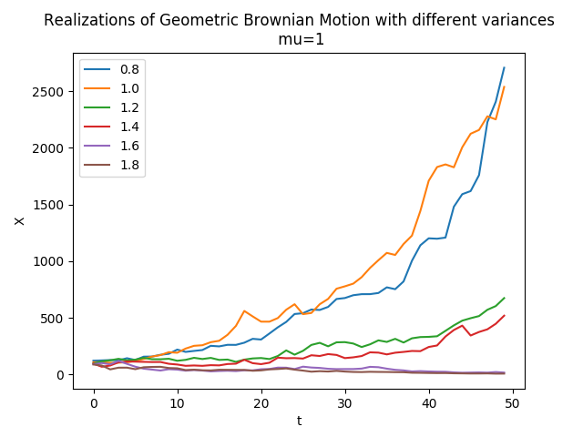
- normally distributed increment additive processes are discrete Brownian processes, financial processes are similar,
- geometrically distributed increment additive processes have negative binomial distributions, e.g. related to random walks, lifetimes,
- exponentially distributed increment additive processes lead to Poisson, e.g. Erlang distributions.
Continuous case: In probability theory, Lévy processes, or additive processes, are continuous stochastic processes with independent, stationary increments. The successive increments are random, in which the increments in pairwise distinct time intervals are independent, and the increments in different time intervals of equal length have the same probability distribution. The Lévy process can be considered the continuous-time analogue of the discrete random walk. The best-known examples of Lévy processes are the Wiener process associated with the normal distribution, and the Brown process associated with the uniform distribution. If the length of the interval t1 - t0 is exponentially distributed, then the process is a Poisson or gamma process.
Discrete case: Even in the discrete case, additive stochastic processes have independent, stationary increments, and
- uniformly distributed increment additive processes have normal distributions,
- normally distributed increment additive processes are discrete Brownian processes, financial processes are similar,
- geometrically distributed increment additive processes have negative binomial distributions, e.g. related to random walks, lifetimes,
- exponentially distributed increment additive processes lead to Poisson, e.g. Erlang distributions.
(https://en.wikipedia.org/wiki/Additive_process, https://en.wikipedia.org/wiki/Independent_increments, https://en.wikipedia.org/wiki/Infinite_divisibility).
Unpredictable white processes have independent events, steps in the future. The Wiener process and white noise are the best known. Among the probability distributions, many probability variables from independent experiments are known, but the distributions with the memorylessness property of geometric, exponential distributions are suitable for describing unpredictable, chaotic systems and processes.
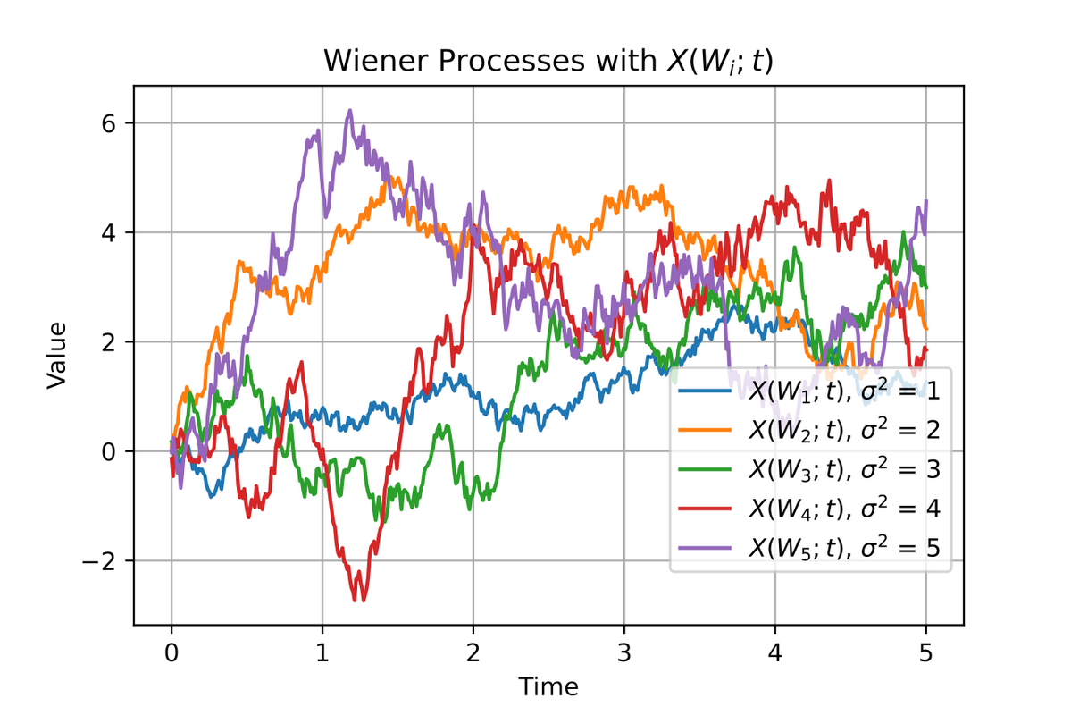
In mathematics, the Wiener process, which is related to wander problems (https://en.wikipedia.org/wiki/Wiener_process), Brownian motion, and the historical physical process of the same name, and is also related to white noise processes. The process is a stochastic process of real-valued, continuous or discrete-time independent increments discovered by Norbert Wiener, where the increments have a normal distribution with zero expected value, and whose derivative process is a white noise process. It is often used in applied mathematics, economics, quantitative finance, evolutionary biology and physics. Properties of the Wiener process t:

- t is a process with independent increments, i. e. for every the increment is independent their past values. When the process is with independent increments if 0 ≤ s1 < t1 ≤ s2 < t2 than Wt1 − Ws1 és Wt2 − Ws2 are independent variables.
- Increments of t have normal distribution,
- The process of t in continuous case: almost certainly in continuous t.


In physics, Brownian motion (https://www.whoi.edu/cms/files/lecture06_21268.pdf) is a continuous, random thermal motion of suspended particles in gases and liquids, discovered by the English botanist Robert Brown when he examined pollen particles mixed with water. The motion was important evidence of the atomic structure of matter. It is a good example of global mixing in chaos theory, whereby, given typical initial conditions, a system will converge to all possible states in a sufficiently long time. The suspended particles undergo constant collisions during their motion, and their behaviour is described by Maxwell's velocity distribution function. Brownian motion trajectories are generally random, continuous and irregular trajectories. Brownian motion is not uncorrelated because the position of a particle at a given instant in time depends on where it was at the previous instant. A characteristic of Brownian motion is that the scattering square increases proportionally with time, so the process is nonstationary, moving away from its initial position proportionally to the square root of time or the number of steps.
White noise (which is a derived process of the Wiener process) is noise whose power density is independent of frequency, i.e. its spectral density is constant over the entire frequency range. The successive noise values are uncorrelated (https://en.wikipedia.org/wiki/White_noise). In reality, there is no infinite bandwidth white noise because it would have infinite power, so we consider band-limited white noise in practice. In numerical simulations, the upper cut-off frequency for sampling is half the sampling frequency. Although the white noise process is uncorrelated, there is a low probability that longer continuous intervals but somewhere can occur with probability 1 in the process, one has not yet seen at band-limited white noise.
Integer walk with random steps
(https://www.mit.edu/~kardar/teaching/projects/chemotaxis(AndreaSchmidt)/random.htm)
A random walk is the process by which randomly moving objects move away from their starting point. There are many types of random walks, such as a stochastic process that consists of random steps over integers, starting at 0 and taking an equal number of steps on the number line with each step taking +1 or −1 steps. Other examples include the path of a molecule as it moves through a liquid or gas (see Brownian motion), the search path of an animal searching for food, fluctuating stock prices, and the financial situation of a gambler. Many processes can be modeled using random walk models, even if these phenomena are not necessarily random in reality. The distance from the starting point is proportional to the square root of the number of steps (https://en.wikipedia.org/wiki/Random_walk). The distance divided by the square root of the number of steps approaches a constant, (2/π)1/2.

The image shows 7 black points starting from the same location with varying step sizes in two dimensions. Pál Erdős and Samuel James Taylor showed in 1960 that in dimensions less than or equal to 4, two independent random walks starting from any two given points will almost certainly have infinitely many intersections, but in dimensions greater than 5, they will almost certainly only intersect finitely often. The asymptotic function of a two-dimensional random walk as the number of steps increases is given by a Rayleigh distribution.
(https://www.mit.edu/~kardar/teaching/projects/chemotaxis(AndreaSchmidt)/random.htm)
(https://www.mit.edu/~kardar/teaching/projects/chemotaxis(AndreaSchmidt)/random.htm)
Random walk (https://en.wikipedia.org/wiki/Random_walk) is a stochastic process, often consisting of random steps on integers, starting at 0, and e.g. with equal probability of +1 or -1 step at each step. Other examples are the trajectory of a molecule as it moves through a liquid or gas (Brownian motion), the search path of an animal looking for food, the prices of fluctuating stocks, and the financial situation of a gambler. Many processes can be modelled using random walk models, even if these phenomena are not necessarily random in reality. It is moving away from its initial position proportionally to the square root of time or the number of steps.

Random walk in two dimension (https://hu.wikipedia.org/wiki/V%C3%A9letlen_bolyong%C3%A1s)
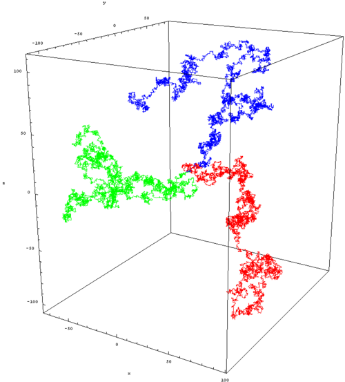
Three dimensional wander, in 1921 György Pólya Pólya proved that for 3 or more dimensions, the probability of returning to the orbit decreases as the number of dimensions increases. In 3 dimensions, the probability decreases to roughly 34%
(https://en.wikipedia.org/wiki/Random_walk)
In higher dimensions, the set of randomly visited points is called a discrete fractal, it is a set that exhibits stochastic self-similarity, yielding spectacular plots in the continuous case. The trajectory of a random walk is the set of visited points, ignoring when the walk visited the point.

When using gradients, we can measure how much the Brownian motion of particles (unit mass/volume) changes as they move from one region to another:
Brownian motion in two dimensions, in gases, in liquids, when the temperature gradient is not yet zero
(https://www.mit.edu/~kardar/teaching/projects/chemotaxis(AndreaSchmidt)/random.htm)
(https://www.mit.edu/~kardar/teaching/projects/chemotaxis(AndreaSchmidt)/random.htm)
Independence, Markov processes, memoryless property
The correlation measures the strength of the linear relationship between two arbitrary values. Uncorrelation does not necessarily mean independence, but it is certain that there is no linear relationship between the values. If the correlation of two random variables is zero, then they are uncorrelated, and the relationship is described by conditional probabilities. It is characteristic of normally distributed random variables that if they are uncorrelated, they are also independent. When the expected value has zero value: the standard deviation of uniformly distributed random variables of white noise can has arbitrary value. Thus the correlation can be used to analyze the strength of the relationship between measurable quantities that can be considered as white noise or normally distributed variables.
Conditional independence: would be a generalization of the independence of events, sets, and random variables using conditional probability and conditional expected value. The conditional expected value is used in probability theory (https://en.wikipedia.org/wiki/Conditional_expectation) to define conditional probability. The conditional expected value can be a random variable or function that is calculated using a conditional probability distribution or, for example, by projecting a vector from the future of the process onto the past of the process, e.g. in realization theory. If the random variable can only take on a finite number of values, then the "condition" is that the variable can only take on a subset of these values. Formally, if the random variable is defined on a discrete probability space, the "conditions" are partitions of this probability space.
Independence: a set of elementary events is pairwise independent if the probability of two events occurring together is the product of the probabilities of the two events, or according to another definition: the conditional probability of an event is equal to the probability of the event. Events that do not occur together, one after the other, form a series. In the series, elementary events are repeated, then the definition of independence is: if the occurrence of an event (or elements) depends only on the last event, element, and is independent of the previous ones, then the series is a Markov process. If the occurrence of an event (or elements) does not depend on either its past or its present, then the process is unpredictable, memoryless, chaotic.
Therefore: In the case of chaotic, unpredictable systems, the distributions used to describe the system can be: the normal, uniform, geometric and exponential distributions, and the distributions and processes derived from them. In the normal and uniform distributions, the expected value and the standard deviation are independent, at the uniform distribution with zero mean its covariance can be arbitrary. The geometric and exponential have memoryless properties, i.e. the future of the process is independent of the present and the past of the process. Note: Relatively few geometric processes can be found in the literature. At negotiation by porjections, the conditional expected value and the noise process associated with chaotic behavior are perpendicular to each other, which allows unambiguous negotiation of unpredictable chaotic systems. The vector of the computed conditional expected value is perpendicular to the estimation error, in the calculation of conditional expected values in the linear case. The assumed noise process is a white Gaussian process or white noise with zero expected value. For exponential or geometric distributions, the past and present of the processes are perpendicular to their future.
In Markov processes, the future of the process depends only on the present of the process. The term Markov process refers to the partially memoryless property of a stochastic process, meaning that its future evolution is independent of its history and depends only on its present. It is named after the Russian mathematician Andrei Markov. In the strong Markov property, the meaning of “present” is defined by a random variable known as the stopping time. A Markov random field extends the property to two or more dimensions.
Distributions, examples of processes
The exponential distribution is often used to model random time periods, waiting times:
- the hereditary property of the exponential distribution models waiting times well,
- the time it takes to serve one person in a shop (queuing theory),
- the time between two customers arriving at a shop,
- the time it takes to perform a calculation on a computer,
- the theory describing traffic situations,
- the reaction time of one person,
- the time between two events occurring, e.g. for incandescent lamps (reliability theory),
- modelling the spread of an epidemic, the spread of an infection, but also the recovery time,
- the decay time of radioactive particles.
A Poisson process (https://en.wikipedia.org/wiki/Poisson_point_process) is a counting process where T1, T2, . . intervals are independent probability variables with exponential distributions. Its basic process is a continuous-time counting process {N(t), t ≥ 0} with the following properties: N(0) = 0, and is characterized by independent increments, stationary increments (the distribution of the number of occurrences in any interval depends only on the length of the intervals) and no simultaneous events. The waiting time for the next event has an exponential distribution. Memoryless i.e. successive arrival events are independent and an event at time t is not affected by any of the events before time t. Applications:
- telephone call arrivals,
- goals scored at football matches,
- requests to web servers.
- particle emission during radioactive decay (which is an inhomogeneous Poisson process),
- queuing theory in which queuing of client-server queues is often a Poisson process.
- telephone call arrivals,
- goals scored at football matches,
- requests to web servers.
- particle emission during radioactive decay (which is an inhomogeneous Poisson process),
- queuing theory in which queuing of client-server queues is often a Poisson process.
The geometric distribution can be used:
- to analyse waiting times before a given event,
- theory describing traffic situations,
- to determine the lifetime of devices and components,
- to determine waiting times until the first failure,
- to determine the number of frequent events between two independent rare events,
- applications such as testing the reliability of devices,
- insurance mathematics,
- to determine the failure rate of data transmission,
- the geometric distribution is the distribution of independent Bernoulli experiments. A generalisation of the geometric distribution is the binomial distribution over several successful trials, which is expressed in two ways: either it is expected to take rth successful trial, or it is emphasised that rth successful trial took n trials. The geometric distribution is a negative binomial distribution for the parameter r=1.
E.g. in queueing theory (https://en.wikipedia.org/wiki/Queueing_theory) the model is constructed so that queue lengths and waiting time can be predicted.
Queueing analysis is the probabilistic analysis of waiting lines, and thus the results, also referred to as the operating characteristics, are probabilistic rather than deterministic. Queueing theory is generally considered a branch of operations research because the results are often used when making business decisions about the resources needed to provide a service, and has its origins in research by Agner Krarup Erlang, who created models to describe the system of incoming calls at the Copenhagen Telephone Exchange Company. These ideas have since seen applications in telecommunications, traffic engineering, computing, project management, and particularly industrial engineering, where they are applied in the design of factories, shops, offices, and hospitals. Consider a queue with one server and the following characteristics:
- : the arrival rate (the reciprocal of the expected time between each customer arriving, e.g. 10 customers per second)
- : the reciprocal of the mean service time (the expected number of consecutive service completions per the same unit time, e.g. per 30 seconds)
- n: the parameter characterizing the number of customers in the system
- : the probability of there being n customers in the system in steady state, and analyzis leads to the geometric distribution formula when λ / μ < 1.


In the one dimensional case, we will consider discrete memoryless series, which are geometrically distributed. If the events of a series are uniformly distributed, with probabilities equal to 1/b, if b is the number of the elementary events, b also denotes the base number of the number system, then some arbitrary k (k=1,2,3,...,kmax) long sequence of the independent elementary events has the probability (b-1)/bk .The parameter of the distribution is (b-1)/b, which is also the probability of a series of unit lengths. The expected value of the distribution is b/(b-1), and the sum of the probabilities has 1 - b-kmax .
Note: For non-countably infinite sequences, the Haar measure (https://en.wikipedia.org/wiki/Haar_measure) is finite in the binary case, i.e. it is a normalizable measure. Although the computation of the Haar measure is complicated, it is an essential statement that there is a measure in the uncountable binary case (because for uncountably infinite sequences the arithmetic mean and the weight are usually divergent). The main queueing models are the single-server waiting line system and the multiple-server waiting line system. These models can be further differentiated depending on whether service times are constant or undefined, the queue length is finite, the calling population is finite, etc.
Note: For non-countably infinite sequences, the Haar measure (https://en.wikipedia.org/wiki/Haar_measure) is finite in the binary case, i.e. it is a normalizable measure. Although the computation of the Haar measure is complicated, it is an essential statement that there is a measure in the uncountable binary case (because for uncountably infinite sequences the arithmetic mean and the weight are usually divergent). The main queueing models are the single-server waiting line system and the multiple-server waiting line system. These models can be further differentiated depending on whether service times are constant or undefined, the queue length is finite, the calling population is finite, etc.
For example, someone's date of birth and random number, in the structure ddmmyy can be retrieved at https://www.piday.org/find-birthday-in-pi/: e.g. 11 January 2011 - the date is '11-11-11', written on the number is in 51150 position in pi, and the number has 9 x10⁻⁶ probability.
Another example: given some pre-recorded text, and a monkey randomly taps the keys of a typewriter indefinitely, it is unlikely that the monkey will eventually write that text, but will do, a mathematical proof of this statement is possible. Cicero argued thus in De natura deorum:
"He who believes this, may also believe that by throwing a bag of twenty-one letters on the ground, the Annales will be read. I doubt if even a short passage of it will appear." Cicero was well aware that the probability of a meaningful text appearing is small, and its possible appearance is inversely proportional to the length of the text. Suppose that the long of the Annales in question is 100 pages long, with 100 letters or signs per page (which is not enough for us, but enough for a monkey). The book contains a total of 10,000 letters or signs. It is indifferent to what it has previously written down for the monkey, since the memoryless property, the distribution is geometric. Let the total number of letters and signs in the typewriter be 30. The probability of each 10,000 long patterns is equal, according to the perpetuity property, i.e. 29 x 30-10000, but where they appear in the sequence we can say nothing about, presumably at long intervals, and with a probability of one, almost certainly (an event with a probability of one is not a certain event, only "almost certain").
"He who believes this, may also believe that by throwing a bag of twenty-one letters on the ground, the Annales will be read. I doubt if even a short passage of it will appear." Cicero was well aware that the probability of a meaningful text appearing is small, and its possible appearance is inversely proportional to the length of the text. Suppose that the long of the Annales in question is 100 pages long, with 100 letters or signs per page (which is not enough for us, but enough for a monkey). The book contains a total of 10,000 letters or signs. It is indifferent to what it has previously written down for the monkey, since the memoryless property, the distribution is geometric. Let the total number of letters and signs in the typewriter be 30. The probability of each 10,000 long patterns is equal, according to the perpetuity property, i.e. 29 x 30-10000, but where they appear in the sequence we can say nothing about, presumably at long intervals, and with a probability of one, almost certainly (an event with a probability of one is not a certain event, only "almost certain").
In the two-dimensional case of plotting random numbers as a function of b, a multidimensional generalization is possible. The images are generated by serializing random numbers, or by assigning a level to each pixel with a random colour generator. Good quality representations of random numbers are indistinguishably similar. Representations of two different random numbers on the coordinates have not been found. When b =2:
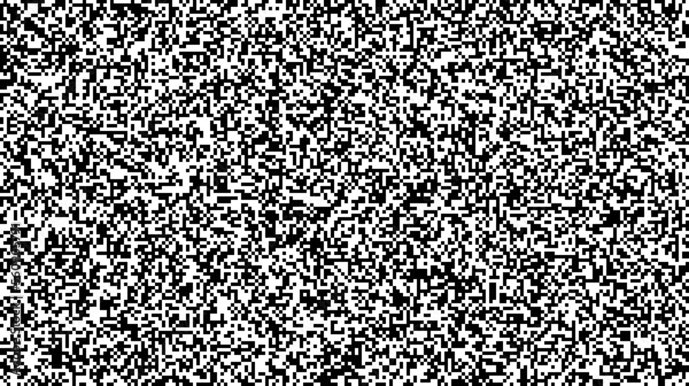
Note that the pattern in two dimensions is a white-black blotch, with mesh-lines in places, and apparently irregular patterns even for higher b values. As the number of pixels increases, there is a small probability that larger black-white patches would appear, corresponding to a decreasing probability that longer sequences would occur in one dimension. Asymptotically, a sample image with the same pixel number can be blacked-out.
If b=3 (white, black, grey)
If b=3 (white, black, grey)

If b= 4 (green, yellow, blue, red)

b = 5 ((green, yellow, blue, red, white)
:

(https://graphicdesign.stackexchange.com/questions/26174/how-can-i-create-a-random-pixelated-pattern, and https://graphicdesign.stackexchange.com/questions/26174/how-can-i-create-a-random-pixelated-pattern)
For graphs (https://ematlap.hu/tudomany-tortenet-2020-11/957-mi-is-az-a-perkolacio): percolation (literally leakage) can be interpreted on any finite or infinite graph, and has two basic variants: in edge percolation, the edges of the graph are drawn independently with probability p equal to the probability of being open or closed by 1-p; in vertex percolation, the vertices are drawn as open or closed. In both variants, the basic phenomena are the same. We think of the closed edges as the ones that we have deleted, and the question is from where to go through the remaining open edges, i.e. what are the remaining random graph's connectivity components. A useful study for leakage models of liquids and gases.
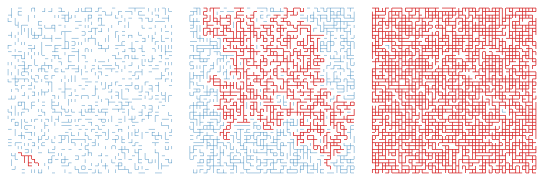
Where can be reached from the open edges for square grid and p=0.25, 0.5, 0.75? The longest path is highlighted in red
*
In the system description in vector space, the future of the process is projected onto the present and past of the process, In the case of an exponential or geometric distribution, the past and present of the processes are perpendicular to their future. The projection vector is the conditional expected value vector calculated with estimates of ARMA model or Kalman filter, to which the unpredictable estimation error vector is perpendicular. The origin of the error vector is Gaussian white noise or uniformly distributed white noise with zero expected value in chaotic systems, memoryless. When the length of the conditional projection vector vanishes, the process is chaotic, which is the mathematical definition of unpredictability, or memoryless. Mathematicians call the conditional expected value estimate (prediction) a filter, engineers call the true value estimate filtering (filtration), the latter means the multiplication of the measured value by the Q/(Q+R) matrix, where R is the measurement noise, Q is the source noise covariance matrix, and Q+R is the covariance matrix of the unpredictable error vector, in the Kalman filter HQHT + R.
Just because a process is a nonstationary stochastic process does not mean that it is unpredictable, nonstationary stochastic processes can often be transformed into stationary ones by transformation. In the simplest examples, they can be eliminated by estimating the trend components (linear, exponential, logistic, periodic...), or by differentiating or forming differences in incremental processes, we can transform the original process into a stationary stochastic process. Nonlinearity can also be handled by linear estimation per section, or if the model is linear in the estimated parameters. The purpose of subtracting the trend components is to finally describe the system with linear models, ARMA or Kalman filters.